Building a Real-Time User Behavior Analytics Pipeline with ClickHouse — From Kafka Ingestion to Materialized Views and Grafana Dashboards
At 1.5 million DAU, the p99 latency of event aggregation queries began exceeding 18 seconds. A single GROUP BY event_type, DATE(event_time) query was consuming over 90% of the CPU on an RDS r5.2xlarge instance, and refreshing the report page directly caused database load spikes. Partitioning and index tuning bought some time, but it was clear that doubling the data would quadruple the response time, not double it.
That's when we took a serious look at ClickHouse. Columnar storage, vectorized execution, and Materialized View-based incremental aggregation were structurally the right fit for this kind of OLAP workload.
This post covers the entire pipeline: ingesting events via Kafka, aggregating them in real time with ClickHouse Materialized Views, and connecting everything to a Grafana dashboard. I'll walk through why we chose this engine, MV design patterns, and the pitfalls you'll encounter in production — honestly. If you've used Kafka before and are evaluating or just getting started with ClickHouse as a backend or data engineer, this should be useful.
Why ClickHouse Fits This Pipeline
Before looking at the code, it makes sense to address "why ClickHouse."
| Item | Details |
|---|---|
| OLAP query speed | Up to 1,000× faster than PostgreSQL on the same data; scans billions of rows in milliseconds |
| Compression ratio | Columnar storage + LZ4/ZSTD achieves 10–20× compression vs. raw, reducing storage costs |
| Concurrent ingest and query | Aggregation queries remain responsive even while Kafka ingestion is running |
| MV incremental aggregation | Aggregating at INSERT time dramatically reduces SELECT load |
| Native Kafka integration | Consume Kafka directly inside ClickHouse — no separate ETL layer needed |
| Horizontal scalability | Built-in sharding and replication; easy cluster expansion |
Real-world adoption backs this up. Wingify (VWO) switched from PostgreSQL to ClickHouse Materialized Views and cut their real-time A/B test aggregation costs by 80%. Braze rebuilt their entire pipeline for hundreds of millions of user behavior events using Kafka → ClickHouse Cloud.
That said, ClickHouse is the wrong tool in some cases. If your workload involves frequent UPDATE/DELETE, JOIN-heavy OLTP patterns, or requires strict row-level Exactly-Once semantics, you should reconsider at the design stage. We'll cover these limitations in the drawbacks section below.
Overall Architecture
The pipeline is divided into three layers: ingestion, storage & aggregation, and visualization.

Kafka durably buffers hundreds of thousands of events per second. ClickHouse stores those events in a columnar structure, and every INSERT triggers a Materialized View that writes aggregated results to a separate table. Grafana queries only the aggregation table, which is why responses become dramatically faster.
The diagram shows that the Kafka Engine path and the Connect Sink path differ. Kafka Engine routes data through an internal Kafka engine table before landing in the raw table, while Connect Sink writes directly to the raw events table without an intermediate engine table.
Core Concepts
Choosing an Ingestion Path: Kafka Engine vs. Kafka Connect Sink

Kafka Engine consumes Kafka topics directly inside ClickHouse. There's no separate ETL layer, which keeps the infrastructure simple. It supports various formats including JSON, Protobuf, and CSV, but automatic Schema Registry integration is only provided for Avro (format_avro_schema_registry_url). Protobuf can be consumed via a local schema file, but there is no built-in support for automatically fetching schemas from a Schema Registry. You should also account for the At-Least-Once guarantee, which can occasionally cause duplicate inserts.
Kafka Connect Sink guarantees Exactly-Once and supports Avro, JSON Schema, Protobuf, and JSON broadly with Schema Registry. Since 2025, Confluent Cloud has also offered a fully managed connector, making the connection configurable entirely through the UI.
For small teams or rapid prototyping, Kafka Engine is the convenient choice. If you need Exactly-Once or Schema Registry-based management for non-Avro formats, Connect Sink is the better fit.
Storage Engine: Choosing from the MergeTree Family
The heart of ClickHouse is the MergeTree engine family.
| Engine | Best For |
|---|---|
MergeTree |
Raw event storage; pure append-only log |
SummingMergeTree |
Simple numeric sum aggregation like counters and totals |
AggregatingMergeTree |
Storing intermediate state for complex aggregates like uniq, avg, and quantile |
ReplacingMergeTree |
Deduplication to complement Kafka at-least-once |
SummingMergeTree is sufficient for simple sums, but aggregations where partial results can't simply be added together — like unique user counts (DAU) or percentiles — require AggregatingMergeTree. This is where the State/Merge pattern comes in, which we'll explain in full in the next section.
How Materialized Views Work
Think of an MV as a trigger + aggregation query that executes synchronously at INSERT time.
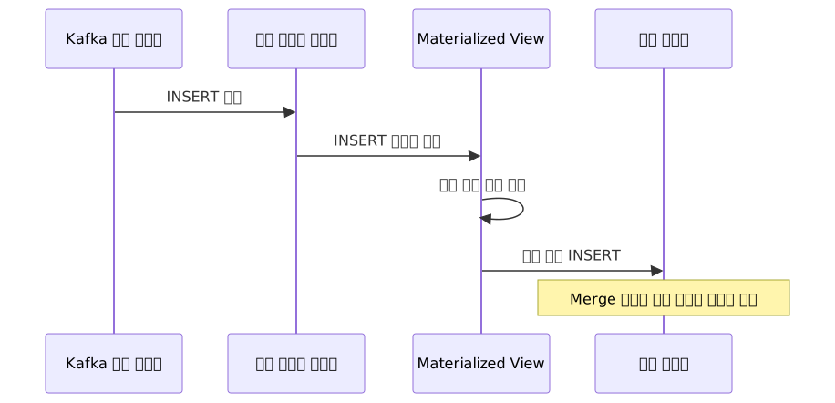
Two key points:
First, an MV runs only against the batch just inserted, not the entire source table. This is what makes incremental aggregation possible.
Second, when reading from an AggregatingMergeTree aggregation table, you must use …Merge functions. When writing, you accumulate intermediate state with …State functions like uniqHLL12State(user_id), and when reading you extract the final value with uniqHLL12Merge(unique_users). Reading State-stored binary values with SUM produces meaningless numbers, and SELECT * will display garbled values directly in your Grafana dashboard. Even if this pattern feels unfamiliar at first, it's precisely why you can roll up hourly aggregates later without double-counting.
Putting It into Practice
The scenario here is an e-commerce service that aggregates click, pageview, and purchase events in real time.
Step 1: Create the Raw Events Table
CREATE TABLE user_events
(
    event_time  DateTime,
    user_id     UInt64,
    session_id  String,
    event_type  LowCardinality(String),
    page_url    String,
    product_id  Nullable(UInt32),
    amount      Nullable(Decimal(10, 2))
)
ENGINE = MergeTree()
PARTITION BY toYYYYMM(event_time)
ORDER BY (event_type, event_time, user_id)
TTL event_time + INTERVAL 90 DAY DELETE;
LowCardinality(String) applies dictionary encoding to low-cardinality string columns, improving both compression ratio and query speed.
ORDER BY (event_type, event_time, user_id) reflects the assumption that "time-range queries per event type" are the most frequent access pattern. If "querying a specific user's activity timeline" is the dominant pattern, (user_id, event_time) would be more efficient. Changing ORDER BY in production requires creating a new table and reinserting all data, so settle this based on your actual query patterns early on.
Step 2: Create the Kafka Engine Table
CREATE TABLE user_events_kafka
(
    event_time  DateTime,
    user_id     UInt64,
    session_id  String,
    event_type  String,
    page_url    String,
    product_id  Nullable(UInt32),
    amount      Nullable(Decimal(10, 2))
)
ENGINE = Kafka()
SETTINGS
    kafka_broker_list       = 'kafka-broker:9092',
    kafka_topic_list        = 'user-events',
    kafka_group_name        = 'clickhouse-consumer',
    kafka_format            = 'JSONEachRow',
    kafka_num_consumers     = 4,
    kafka_max_block_size    = 65536,
    kafka_handle_error_mode = 'stream';
kafka_max_block_size is the maximum number of messages to fetch from Kafka in one batch. The default (65536) balances throughput and latency, but you can increase it if messages are large or some ingestion delay is acceptable. Since it directly affects INSERT batch size and MV execution frequency, benchmark it against your environment.
kafka_handle_error_mode = 'stream' prevents the consumer from stopping on parse failures; instead, it exposes error details via the _error and _raw_message virtual columns. Routing these columns to a separate MV implements a Dead Letter Queue (DLQ) pattern.
The Kafka Engine table itself does not serve as permanent storage. Data must be forwarded to the raw events table via the MV in the next step.
Step 3: MVs to Route Kafka into the Raw Table and DLQ
An MV that routes valid messages to the raw table:
CREATE MATERIALIZED VIEW user_events_ingest_mv
TO user_events
AS
SELECT
    event_time,
    user_id,
    session_id,
    event_type,
    page_url,
    product_id,
    amount
FROM user_events_kafka
WHERE _error = '';
A DLQ table and MV that preserve messages that failed to parse:
CREATE TABLE user_events_dlq
(
    raw_message String,
    error       String,
    received_at DateTime DEFAULT now()
)
ENGINE = MergeTree()
ORDER BY received_at
TTL received_at + INTERVAL 7 DAY DELETE;

CREATE MATERIALIZED VIEW user_events_dlq_mv
TO user_events_dlq
AS
SELECT
    _raw_message AS raw_message,
    _error       AS error
FROM user_events_kafka
WHERE _error != '';
With this structure in place, malformed messages won't stop the consumer. Error messages can be inspected and reprocessed from the user_events_dlq table, and the pipeline keeps flowing without any manual offset skipping.
Step 4: Hourly Aggregation with AggregatingMergeTree
An example of aggregating session counts and unique user counts per hour and event type in real time:
CREATE TABLE user_events_hourly_agg
(
    hour          DateTime,
    event_type    LowCardinality(String),
    session_count AggregateFunction(uniq, String),
    unique_users  AggregateFunction(uniqHLL12, UInt64)
)
ENGINE = AggregatingMergeTree()
ORDER BY (hour, event_type);

CREATE MATERIALIZED VIEW user_events_hourly_mv
TO user_events_hourly_agg
AS
SELECT
    toStartOfHour(event_time) AS hour,
    event_type,
    uniqState(session_id)     AS session_count,
    uniqHLL12State(user_id)   AS unique_users
FROM user_events
GROUP BY hour, event_type;
It's worth noting why uniqState(session_id) is used for session_count instead of countState(). countState() counts the number of rows in an INSERT batch — i.e., the number of events. If multiple events come in from the same session, each is counted separately, producing a value completely different from the actual session count. uniqState(session_id) tracks the number of distinct session_id values. The column type must also match: AggregateFunction(uniq, String).
When reading, use …Merge functions:
SELECT
    hour,
    event_type,
    uniqMerge(session_count)      AS total_sessions,
    uniqHLL12Merge(unique_users)  AS dau
FROM user_events_hourly_agg
WHERE hour >= now() - INTERVAL 24 HOUR
GROUP BY hour, event_type
ORDER BY hour DESC;
Step 5: Daily Purchase Sum Aggregation with SummingMergeTree
For simple sums, SummingMergeTree is much more straightforward:
CREATE TABLE purchase_daily_sum
(
    day            Date,
    product_id     UInt32,
    total_amount   Decimal(18, 2),
    purchase_count UInt64
)
ENGINE = SummingMergeTree((total_amount, purchase_count))
PARTITION BY toYYYYMM(day)
ORDER BY (day, product_id);

CREATE MATERIALIZED VIEW purchase_daily_mv
TO purchase_daily_sum
AS
SELECT
    toDate(event_time) AS day,
    product_id,
    sum(amount)        AS total_amount,
    count()            AS purchase_count
FROM user_events
WHERE event_type = 'purchase' AND product_id IS NOT NULL
GROUP BY day, product_id;
total_amount is declared as Decimal(18, 2) to prevent summation overflow. The source amount is Decimal(10, 2), capping a single transaction at roughly 99,999,999.99, but accumulating millions of purchases daily can easily exceed this range. It's safer to use a generous precision in aggregation tables.
SummingMergeTree automatically sums numeric columns when merging rows with the same ORDER BY key. To get accurate totals that include not-yet-merged parts, always read with GROUP BY + sum().
SELECT
    day,
    product_id,
    sum(total_amount)   AS total_revenue,
    sum(purchase_count) AS orders
FROM purchase_daily_sum
WHERE day >= today() - 30
GROUP BY day, product_id
ORDER BY total_revenue DESC;
Grafana Connection Configuration
apiVersion: 1
datasources:
  - name: ClickHouse
    type: grafana-clickhouse-datasource
    jsonData:
      defaultDatabase: default
      protocol: native
      server: clickhouse-server
      port: 9000
      username: default
    secureJsonData:
      password: ""
username belongs in jsonData. secureJsonData is the section reserved for values that must not be stored in plain text (like password), so placing username there will not work as intended.
The native protocol (port 9000) is slightly faster than HTTP (port 8123). Starting with plugin v4, a built-in log and trace query builder is included, allowing SREs and data analysts to build dashboards without writing SQL.
An example time-series query for a dashboard panel querying the aggregation table:
SELECT
    hour AS time,
    event_type,
    uniqHLL12Merge(unique_users) AS dau
FROM user_events_hourly_agg
WHERE hour >= $__fromTime AND hour <= $__toTime
GROUP BY time, event_type
ORDER BY time ASC;
The hour column already holds values aggregated by toStartOfHour(). Applying toStartOfMinute() to it would just repeat the same timestamp — it does not provide minute-level granularity. If you need per-minute aggregation, query the raw events table directly or create a separate minute-level aggregation table. Grafana's $__fromTime and $__toTime macros automatically bind the dashboard time range filter.
Production Drawbacks and Pitfalls
Limitations to Be Aware Of
| Item | Details |
|---|---|
| At-Least-Once guarantee | Kafka Engine can occasionally produce duplicate inserts; use ReplacingMergeTree or design for idempotency |
| MV INSERT blocking | MVs execute synchronously with INSERTs, so many complex MVs can cause ingestion delays |
| High-cardinality limits | Very high unique value counts in GROUP BY keys cause the target table to bloat, negating performance gains |
| Difficult schema changes | Changing an MV target table's schema requires a blue-green approach: create a new table and MV, then cut over traffic |
| Limited Schema Registry support | Kafka Engine's automatic Schema Registry integration only supports Avro; use Connect Sink for non-Avro formats with Schema Registry |
| Inefficient JOINs and updates | Optimized for append-only workloads; not suitable for frequent UPDATE/DELETE or complex JOINs |
| Learning curve | Engine selection, partition design, and TTL settings directly impact performance; initial design costs are high |
Two Common Pitfalls in Practice
① Underestimating the cost of schema changes
ORDER BY, PARTITION BY, and data types cannot be changed via ALTER in production, or require a full table rebuild. If you don't carefully examine data volume and query patterns up front, you'll find yourself reinserting billions of rows into a new table. Wingify publicly noted that an early partitioning mistake required significant repartitioning effort. The design time you invest early is far cheaper than a later rebuild.
② Reading aggregation tables with SELECT *
Querying an AggregatingMergeTree table with SELECT * returns raw binary state values. You must use …Merge functions to get human-readable results. If you're seeing strange numbers or NaN in Grafana, this is most likely the reason.
Closing Thoughts
Here's a summary of the key takeaways from this post:
- For the Kafka → ClickHouse connection, choose between Kafka Engine and Connect Sink based on whether you need Exactly-Once and Schema Registry integration. Kafka Engine is simpler to operate and supports various formats including JSON, but if you need Exactly-Once or Schema Registry for non-Avro formats, Connect Sink is the right choice.
- Configuring a DLQ pattern with
kafka_handle_error_mode = 'stream'ensures that malformed messages don't stop the consumer and are instead routed to a separate error table. - Use SummingMergeTree for simple sums and AggregatingMergeTree for complex aggregates like unique counts and percentiles. The core pattern is storing with
…Stateand reading with…Merge; also make sure column names accurately reflect what's actually being computed. - Materialized Views are INSERT triggers, which lets you maintain aggregation tables in real time with virtually no SELECT load. High MV complexity translates into ingestion delays, so find the right balance at design time.
- Starting with Grafana plugin v4, the built-in query builder lets analysts build dashboards without writing SQL.
If you want to get started right now, here's a suggested approach:
- Spin up a cluster on the ClickHouse Cloud free tier, INSERT a sample events CSV, and get a direct feel for MergeTree and aggregation query speed.
- Set up Kafka + ClickHouse locally with Docker Compose, connect a Kafka Engine table to a simple Materialized View, and watch the event flow in action.
- Connect Grafana and build a single time-series panel using a
$__fromTimemacro query to get an end-to-end feel for the full pipeline.
In ClickHouse, initial design decisions have an outsized impact on long-term operational costs. Changing ORDER BY, PARTITION BY, or TTL settings in production can mean rewriting billions of rows. Taking the time to thoroughly understand your data volume and query patterns before you start will pay significant dividends by avoiding costly redesigns later.
References
- ClickHouse Official Kafka Integration Docs
- ClickHouse Materialized View Best Practices (Official)
- Grafana ClickHouse Observability Official Guide
- Grafana Labs Official ClickHouse Plugin
- ClickHouse 2025 Annual Roundup
- How Braze Rebuilt Their Real-Time Analytics Pipeline with ClickHouse Cloud
- Wingify: 80% Aggregation Cost Reduction with Materialized Views
- Comparing 3 Kafka → ClickHouse Ingestion Methods
- Complete Guide to ClickHouse Materialized Views (GlassFlow)
- Announcing Fully Managed ClickHouse Connector on Confluent Cloud
- AggregatingMergeTree In Depth
- ClickHouse Kafka Engine vs. Tinybird Connector Comparison
- Simplifying Real-Time Pipelines: How ClickHouse Replaced Flink for Kafka Streams
- Real-Time Click Stream Analytics GitHub Repo